The previous chapter introduced two new algorithms for the stream compiler. The stream compiler transforms the source code into an executable, performing optimisations using the information known before the program starts running. This chapter focuses instead on the decisions taken at run time. In particular, this chapter is concerned with dynamic scheduling of stream programs.
A program can be scheduled either statically, by the compiler, or dynamically, by the run-time system. Chapter 3 was concerned with static scheduling. If the program is scheduled statically, each task becomes a thread containing a loop, each iteration of which executes its kernels’ work functions in sequence. Tasks communicate using communications primitives, which they call as and when they need them. This implies a relatively simple run-time system, similar to acolib. The main advantages of static scheduling are low overhead and low memory use.
If the program is scheduled dynamically, each task is broken up into self-contained, non-blocking tasks. The dynamic scheduler decides in which order to run these tasks, constrained by dependencies between them: a task cannot start if it needs an output from a task that hasn’t yet finished. Tasks consume input when they start and produce output when they complete, rather than communicating as required using communications primitives.
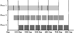
Dynamic scheduling is the only choice when the program’s behaviour is unpredictable. It also supports stream graphs that are not known at compile time, because kernels and streams are introduced dynamically. As illustrated in Figure 4.1, a dynamic scheduler adds overhead, but it can be better overall when the partitioned stream program is unbalanced. The discussion in Section 4.2.2 gives an example.
A dynamically scheduled program still benefits from unrolling and partitioning transformations, since they coarsen the granularity, and bigger tasks have smaller total overhead. In addition, unrolling enables vectorisation, and task fusion enables data reuse and polyhedral transformations. A partitioning transformation for a dynamic scheduler, unlike the algorithm in Chapter 3, does not need to map tasks to processors.
Section 4.1 defines the dynamic scheduling problem. Section 4.2 describes the previously known scheduling algorithms, and gives a worst case example for each. Section 4.3 develops an adaptive scheduler for stream-like applications. There are two variants of this scheduler, the apriority stream scheduler requires a one-dimensional stream program, and it needs annotations from the compiler. The gpriority general-purpose scheduler is more general, and it does not need any additional information. Section 4.4 is the experimental evaluation.
Figure 4.1: Example traces with static and dynamic scheduling (black is scheduling overhead and shades distinguish kernels)
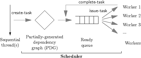
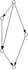
The stream program starts executing on one processor, in a sequential master thread. Whenever the master thread reaches a function marked as a task, the function does not execute right away. Instead, an instance of that task is created, and added to the partially-generated dependency graph (PDG). The PDG holds tasks until they have finished executing. Each vertex is a task, and each directed edge represents a dependency between tasks. When the predecessors of a task, if any, have all finished, the task becomes ready. Ready tasks are held in a data structure known as the ready queue, until they are issued, in an order determined by the dynamic scheduler. Figure 4.2 illustrates this process, showing the dynamic scheduler in context.
The dynamic scheduler supports the three operations labelled in Figure 4.2:
| void create-task(Task task-id, Task-set preds) |
| Task issue-task(Worker worker) |
| void complete-task(Task task-id) |
-1 The create-task operation adds a task to the partial dependency graph (PDG). Its arguments identify the task, and the set of tasks whose outputs it consumes. The issue-task operation is called by a worker when it is idle; it waits for and returns the next ready task to issue. The complete-task operation is called by a worker when it finishes executing its task; it notifies the scheduler that the outputs from that task are now ready. A complete scheduler would provide some additional operations, to support initialisation, barriers, and so on, but they are not relevant here. This interface is similar to the interface between Nanos++ [Nana] and its scheduler plugin.
-1 This construction has some direct implications. First, tasks are non-preemptive, so once issued, they run to completion. Second, the scheduler is non-clairvoyant, meaning that task execution times are not known until they complete. Third, the dependency graph is built by a sequential thread, and is not known all at once.
Another aspect of scheduling is the throttle policy. The program may create a large number of tasks in the course of its execution, so the main thread should be stalled if the PDG contains too many tasks. On Nanos++, this is done by inlining the next task, effectively making the rest of the master thread a new task dependent on the newly created one. This is a reasonable way to prune a recursive computation such as quicksort, which would otherwise create a large number of very small tasks. On CellSs, the main program on the PPE simply stalls, and the processor does not become an extra worker, since all the workers are SPEs.
The decision to stall task creation is taken by the throttle policy. In Nanos++, the default throttle policy is based on the number of ready tasks per processor, inlining tasks if the number of ready tasks is greater than some threshold.
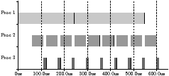
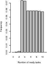
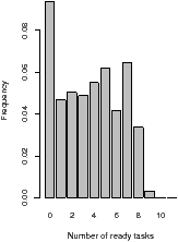
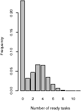
For one-dimensional stream programs, the number of ready tasks is usually confined to a relatively narrow region, as shown in the histograms in Figure 4.3. These histograms show the distribution of the number of ready tasks, sampled at a constant rate. If the threshold is greater than ten, it is never exceeded, and the size of the PDG will grow without limit. If it is less than ten, the main thread will stall too frequently. A better throttle policy is one based on the number of tasks in the PDG. The main thread should be stalled when the PDG contains a certain number of iterations’ worth of tasks.
The precise goal of the scheduler depends on the context. An offline stream program, such as video transcoding or a database query, should be finished as soon as possible. In standard terminology, the scheduler’s objective would be to minimise the makespan, written Cmax, the time that the last task finishes.
Other stream programs, such as video playback, operate in real time. This suggests that an additional goal should be to minimise latency, so that an output frame isn’t delayed by the processing of too many tasks from future frames.
An additional constraint on the scheduler is memory footprint. If the memory footprint is too large, either performance will suffer through paging to disk, or the program will fail due to insufficient memory.
The scheduling problem is NP-hard, because it includes a well-known NP-hard problem as a special case. This corresponds to the case where the dependency graph is known up-front, a problem known as p | prec | Cmax [LK78, Ull75].1 The scheduler therefore has to use a heuristic, which tries to find a good solution that might not be optimal. Many heuristics have been proposed, for various related scheduling problems, and a selection is given in Table 4.1. Many of these heuristics are unsuitable because they require the task execution times, they need to schedule the whole program in advance, or they are too slow.
Abbrev. Full name Year Online? Heterogeneous? Clairvoyant Note HLFNET [ACD74] Highest Levels First with No Estimated Finish Times 1974 Offline Homo No Same as botlev SCFNET [ACD74] Smallest Co-levels First with No Estimated Finish Times 1974 Online Homo No Same as toplev DSH [KL88] Duplication Scheduling Heuristic 1988 Offline Homo Yes O(n4) is too slow ETF [HCAL89] Earliest Task First 1989 Online Homo No Schedules task that would start first MCP [WG90] Modified Critical Path 1990 Offline Homo Yes Like botlev, but takes account of descendants’ bottom levels MH [ERL90] Mapping Heuristic 1990 Offline Hetero Yes O(n2p3) is too slow GDL [SL93] Generalised Dynamic Level 1993 Offline Hetero Yes DSC [YG94] Dominant Sequence Clustering 1994 Offline Homo Yes BIL [OH96] Best Imaginary Level 1996 Offline Hetero Yes HEFT [THW99] Heterogeneous Earliest Finish Time 1999 Offline Hetero Yes MCT [MAS+02] Minimum Completion Time 1999 Online Hetero Yes MET [MAS+02] Minimum Execution Time 1999 Online Hetero Yes PCT [MAS+02] Partial Completion Time 1999 Online Hetero Yes OLB [MAS+02] Opportunistic Load Balancing 1999 Online Hetero Yes CPOP [THW99] Critical Path on a Processor 1999 Offline Hetero Yes k-DLA [WY02] k-Depth Lookahead 2002 Offline Hetero Yes HCPT [HJ03] Heterogeneous Critical Parent Trees 2003 Offline Hetero Yes
Table 4.1: Known DAG scheduling heuristics, related to the problem in this chapter
This section investigates the performance of the scheduling algorithms listed in Table 4.2. These policies are non-preemptive, non-clairvoyant, online, and fast. The next subsection describes the policies in detail. Subsection 4.2.2 gives a simple realistic worst-case example for each policy. Subsection 4.4 is an empirical analysis on a 16-core machine.
Table 4.2: The scheduling policies and cost, where W is the number of tasks in the PDG, and R is the number of ready tasks
Table 4.2 lists the scheduling policies investigated in this section. All policies work by issuing a ready task with the highest priority, where the priorities may be adjusted dynamically, and they differ, of course, between the policies. It is possible to construct examples that cannot be scheduled optimally by any priority-based scheduler [Koh75], since the optimal schedule may require unforced idle time: a processor waiting idle for some time, even though there are some ready tasks. Section 4.2.2 gives an example stream program, observed in practice, which has poor performance for this reason, when using the oldest-first scheduler.
The fifo (first in–first out) policy schedules the task that became ready first. Conversely, the lifo (last in–last out) policy schedules the one that became ready last. For recursively generated computations, such as quicksort, fifo tends to open up parallelism, because it schedules larger tasks near the top of the call tree first, doing the computation in breadth-first order. In contrast, lifo has lower memory use and better data locality, and would often be the best schedule for a single processor. The Cilk scheduler [BJK+95] uses LIFO for local queues and FIFO for work stealing.
The oldest policy schedules the task that was created first. This policy is similar to FIFO when all tasks are independent.
The remaining policies use the metrics illustrated in Figure 4.4. The toplev policy schedules a task with the minimum top level; the top level is the number of edges in a longest path from a source vertex to the task. Similarly, the botlev policy schedules a task with the maximum bottom level, which is the number of edges in a longest path from the task to a sink vertex. The toplev and botlev policies are also called SCFNET and HLFNET, respectively [ACD74]. The botlev policy was used for task scheduling in 1969 [Bow69], and later, when taking account of known computation times, it was known as HLFET and the Critical Path Method.
There is an important difference between the top and bottom levels. The top level is easily calculated in task creation, and is then known for certain, but the bottom level must be calculated bottom up. Adding a task to the PDG may change the bottom level of every other task. The average case will normally be less expensive, since the traversal can terminate whenever it reaches a task whose bottom level is not changed. The bottom levels may be updated in this way, either every time a task is created, or periodically.
The crit policy schedules a task with the maximum criticality, which is the sum of the top and bottom levels. The crit policy is equivalent to choosing a task with the least slack (sometimes called the mobility). The mchild policy schedules a task with the greatest number of successors. The aim is to try to open up parallelism, but the policy is short-sighted because it is local, and it is not adaptive, because it keeps opening up parallelism even if there is plenty enough already. The mdesc policy schedules a task with the greatest number of descendants. It is expensive and has poor performance.
The wave scheduler is specific to one dimensional stream programs. It schedules a kernel with lowest wave number, where the wave number of a kernel is equal to the iteration number plus the kernel’s top level within the iteration. It is equal to the top level when all kernels have multiplicity one.
The apriority and gpriority policies are the adaptive schedulers that will be introduced in Section 4.3. The results are presented in this section so they can be more easily compared with the existing schedulers.
All policies except oldest-first may give several tasks the same priority. Often the tie will be broken in some arbitrary way, but this could be done using a second scheduling policy. Continuing like this, a heuristic is a list of policies; e.g. (fifo, oldest) is a FIFO scheduler, but if several tasks became ready at the same time, they are scheduled in increasing order of their creation time.
Table 4.2 summarises the overall amortised per task time complexity of the policies. The complexity takes account of the cost of assigning priorities, updating priorities when other tasks are created, and pushing and popping tasks to the ready “queue”.
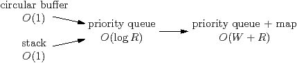
The table shows the ready “queue” data structure required by each policy. The fifo policy, on its own, simply uses a circular buffer for the ready queue. There is no need to explicitly track priorities, because the priority of a task is known when it becomes ready, and is implied by its position in the circular buffer. Similarly, lifo uses a stack. For fifo and lifo, insertion and removal are both constant time: O(1).
The oldest, toplev and wave policies use a priority queue, because the task’s priority is known at creation time, and therefore known at ready time, when the task is inserted into the queue. Similarly for apriority and gpriority. Both insertion and removal have cost O(logr), using a heap or self-balancing binary tree, where r is the current size of the ready queue. The average value of logr is written logR. In both cases, calculating the priority itself is constant time: O(1), so overall the cost per task is logR.
For the remaining policies, task priorities are not known until issue time, but a lower bound is known at ready time. For example, the mchild policy schedules the task with the greatest number of children. When a task becomes ready, some of its children may already have been created, but not always all of them. Each time another task is created, all of its parents require their priority to be increased by one. The number of ready parents is at most the number of function arguments, so the extra number of updates per task is O(1).
These policies can be implemented using a priority queue, since priority queues typically provide an operation that increases an element’s priority. It also requires a map from the task ID to its position in the priority queue; e.g. the node in a tree, and this map must be updated as the priority queue is manipulated. Task removal has cost O(logr), as before, but task creation requires some of the priorities of the tasks in the ready queue to be updated. Using a balanced tree or heap, updating the priority of a single task in the ready queue is O(logr); using a Fibonacci heap, it is O(1) amortised time [FT87a].
For botlev, crit, and mdesc, adding a single task may change the priority of every other task in the PDG. There are simple, common, examples, for each of the three policies, that exhibit this worse case.
A heuristic is a list of policies, and the ready queue for a heuristic is the most general of the ready queues of its policies; i.e. the one that is furthest to the right of Figure 4.5.
Throughput (compared with optimal)
Table 4.3: Throughput for one dimensional stream programs, compared with optimal, where p is the number of processors, f is the unroll factor, f* = p−1/f, f†= p−1/f+1
This section exhibits simple, realistic worst case examples for the scheduling heuristics. Many of these examples occur in the results in Section 4.4. All the examples are one-dimensional “streaming” programs, constructed by a single for loop containing calls to several kernels. Each such call generates a task. The multiplicity, or number of tasks per kernel per iteration, varies between kernels.
These streaming examples divide into two groups, which correspond to the two main ways that the schedule can be bad. The first group suffers from exhaustion, meaning that the scheduler frequently runs out of parallelism throughout the execution. This happens when the scheduler tends to complete all the kernels from one loop iteration before starting the next iteration. This is typical of oldest, and it is inappropriate when the next iteration begins with a long kernel, on which all other kernels depend.
-1 The second group suffers from poor back pressure, meaning that some kernels execute the loop iterations at a faster rate than others. Poor back pressure implies poor temporal data locality, which, if the amount of data transferred between kernels is large, will reduce performance significantly. If the amount of data transferred is small, when all iterations of the faster kernels have been done, there may not be enough parallelism left to keep all of the processors busy. Back pressure can be helped by reducing the window size, but it still uses more memory than it should; exhaustion cannot.
Table 4.3 shows the worst case throughput, as a multiple of the optimal throughput. These figures assume that the number of iterations are large, so they exclude the overhead at the start and end of the program. All examples have an optimal schedule with all processors 100% busy during the steady state.
Many examples have worst case ratio close to p/2p−1, so for large numbers of processors, on average they use only half of the number of processors as the optimal schedule. Graham’s bound [Gra71] shows that any demand scheduler; i.e. one using priorities or a list schedule, has execution time at most 2p−1/p times optimal; so this bound is indeed the worst case.
These examples are synchronous dataflow (SDF) [LM87] streaming programs, so they could also be scheduled statically, at compile time. Table 4.3 shows the worst case for optimal static schedulers with and without support for kernel fission, which splits stateless kernels (a kernel is stateless if there is no dependency path from one iteration of the kernel to another).
If the static scheduler does not support fission, the worst case is when most of the work is in a single stateless kernel, since the static scheduler allocates that kernel to one of the processors, while any dynamic scheduler would run it on them all. With kernel fission, the worst case is a pipeline of p+1 stateful kernels. One processor must be assigned two of them, giving utilisation p+1/2p, which approaches one half for large p.
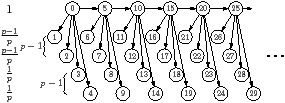
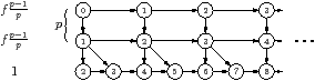
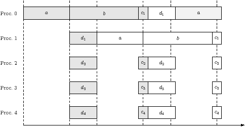
Figure 4.6(a) is an example where the oldest policy suffers from exhaustion. The iterations of the loop run from left to the right. Each row is a kernel, all of whose tasks have the same execution time, shown to the left of the diagram. The vertex labels, for this one diagram, number the tasks in the order they were created. The other diagrams will highlight whichever metric is used by the scheduler. The diagram is illustrated for p=3 processors.
An optimal schedule allocates one processor to the top row, at cost 1 per iteration. The remaining p−1 processors are each allocated to one row of cost p−1/p and one row of cost 1/p, for a total cost per processor also equal to 1 per iteration. The schedule is a pipeline of length two, and the loads are balanced, so steady state utilisation is 100%.
-1 The oldest scheduler will first issue task 0 from the top row. Once that has completed, all other tasks in the same iteration (1, 2, 3, and 4 in the picture) become ready. The next task from the top row, 5, also becomes ready, but it will not be issued until the tasks from the same iteration have been done. The kernel execution times have been chosen so that all processors finish the first iteration at the same time. At this point, the first task, 5, in the next iteration can start on one processor, but the remaining processors will be idle.2 Each iteration requires time 1 for the task from the top row, plus time p−1/p for the remaining tasks; hence the result in Table 4.3.
This example is a perfectly ordinary stream program, and several StreamIt benchmarks suffer a similar fate. The fm benchmark illustrated in is a good example.
This example can be adapted for some of the other heuristics. It works as it stands for (fifo, oldest) and (lifo, oldest), because in the above description, all tasks in the ready queue became ready at the same time. To produce a general example for fifo and toplev, add a zero-cost task between each consecutive pair of tasks in the top row; i.e. between tasks 0 and 5, and 5 and 10; and so on.
-1 Figure 4.6(b) shows a similar example for botlev and crit. The labels inside the tasks are the bottom level, and the labels outside are the criticality. The analysis is the same as before, and this example also turns up in the empirical analysis. Similar examples exist for mchild and mdesc. A possibility for the latter is to unroll all but the first kernel and make the branches of the split stateful; this is one of many ways to ensure that the branches of the split have more descendants than the next task in the top row.
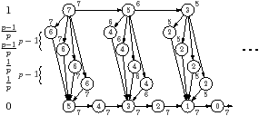
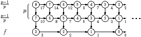
Figure 4.7(a) is an example where toplev suffers from poor back pressure. Each task is labelled with the top level. There are p+1 kernels, the first p of them with multiplicity one, and the last with multiplicity f. The diagram is illustrated for p=2 processors, and f=2. The first p rows have tasks of cost f(p−1)/p, after unrolling, and the final row has tasks of cost 1.
An optimal dynamic schedule uses p−1 processors for the top p rows, and the remaining processor for the bottom row. The bottom row has cost 1 per iteration of the original loop. The tasks in the top p rows each have cost f(p−1)/p, but they each cover f iterations of the original loop. Hence the total cost for f iterations of the top p rows is f(p−1), which is also 1 per processor per original iteration. Ignoring the first few and last few iterations, the load is balanced perfectly, and can be scheduled as a pipeline, so utilisation is 100%.
The toplev scheduler proceeds by top level, with 100% utilisation until the last task in the top row has been completed. At that point, the top p rows are all close to complete, but the bottom row is about 1/f complete. The rest of the bottom row will be serialised.
For n complete iterations of the original loop, the total busy CPU time, for either scheduler, is np. The toplev scheduler has idle time equal to
| t = (p−1)n | ⎛ ⎜ ⎜ ⎝ | 1− |
| ⎞ ⎟ ⎟ ⎠ | , |
since p−1 processors wait for the completion of the bottom row.
The ratio of total time is therefore
|
For large unroll factors, the relative utilisation is close to p/2p−1, itself close to one half for large numbers of processors.
-1 Figure 4.7(b) is a similar example for botlev and mdesc. The labels inside the tasks are the bottom level, and the labels outside are the number of descendants. The analysis is similar to the previous case, leaving much of the bottom row to be processed sequentially on one processor. For botlev, the bottom row will not be started until only 1/f of the top row is left. At this point, the p+1 rows will be processed together, until just the bottom row is left. For mdesc, the bottom row will begin execution a little later, but the analysis is similar.
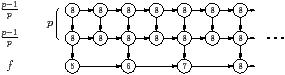
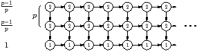
-1 Figures 4.7(c) and (d) show worst-case examples for crit, and mchild and lifo. The labels inside the tasks are the priorities, given by the criticality and number of children, respectively. In both cases, none of the tasks from the bottom row will be issued until the top row is finished. For crit, this is true whatever the unroll factor, because removing just one task from the bottom row moves the bottom row off the critical path. For mchild, this is true because the tasks in the bottom row have one child, whereas all the other tasks have two.
For lifo, the first or second task in the bottom row will be delayed until the end of the execution, because it will always have been the first task put in the ready queue that has still to be done.
For fifo, the utilisation under exhaustion is slightly higher, at 2p/3p−1. An example is a stateful pipeline, similar to Figure 4.7(d), but with p(p−1) kernels of cost 1, followed by a single high-cost kernel of cost p+є, for small є. An optimal schedule has a perfectly balanced pipeline, processing one iteration every p time units.
The fifo schedule, however, runs the high cost kernel at one half the rate of the other kernels. The remaining iterations of this kernel will have to be processed on one processor. This is because while a high-cost task is executing, a complete wave of other tasks can complete: in time p on p−1 remaining processors, p(p−1) tasks are completed. When the high-cost task has completed, there is a whole new wave of other tasks in the FIFO queue ahead of it, so a second wave completes before the next high-cost task starts. The utilisation, in Table 4.3, is like toplev with f=2.
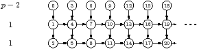
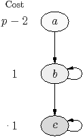
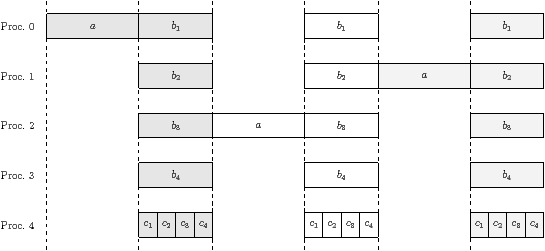
Surprisingly perhaps, the oldest scheduler can also suffer from poor back pressure. This is possible, even though it always assigns highest priority to the oldest task. An example is shown in Figure 4.7(e). This example is redrawn in Figure 4.8(a) as a stream graph, with the kernels labeled a, b, and c.
The costs are chosen so that the optimal schedule should use, on average, one processor for kernel b, one processor for c, and the rest of the processors for kernel a.
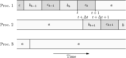
In fact, the oldest scheduler often uses one processor for both b and c, and p−1 instead of p−2 processors for the rest, causing the back pressure problem. Figure 4.8(b) shows why. When processor 3 finishes a task, processor 1 is currently executing an iteration of kernel b, and no iterations of either kernel b or c are ready. It therefore has to execute another iteration of kernel a. When processor 2 finishes its task, processor 1 is currently executing kernel c, and the next iteration of kernel b is ready. This allows processor 2 to begin executing this kernel, opening up parallelism. However, when processor 1 finishes, the only ready tasks are again those from kernel a. The overlap is therefore short-lived, and only in exceptional runs are there are a significant amount of concurrency between kernels b and c.
This section describes two adaptive schedulers for stream-like programs. The first, adaptive priority (apriority), is specific to one-dimensional stream programs. The second, general adaptive priority (gpriority), has slightly more overhead but it is more general.
Both policies are low overhead, and are based on the oldest-first scheduler. As will be seen in Section 4.4, oldest-first has the lowest memory use, and it usually has the best performance, but it sometimes suffers from exhaustion. The adaptive schedulers modify the oldest first scheduler so that if exhaustion occurs, the priorities are adjusted to try to stop it happening again. If exhaustion never happens, both policies remain the same as oldest throughout execution, retaining its low memory use.
The oldest scheduler issues the task with the smallest task number; that is, the priority is zero minus the task number. Both the adaptive schedulers modify this priority by adding an adjustment, which depends only on the kernel ID. The adjustments start at zero. Whenever a kernel is seen to be a bottleneck, the adjustments of that kernel and its ancestors are increased.
Both adaptive schedulers have complexity similar to that of oldest-first. They hold the ready tasks in a priority queue, which has complexity per task equal to the average value of the logarithm of the number of ready tasks. Ready tasks are inserted with known priority. The schedulers maintain a small table of metrics, described later, which is updated in constant time per task. The priority adjustments are updated infrequently, and the cost is linear in the number of kernels. In addition, the gpriority scheduler has some overhead at task creation time, which has a constant cost per dependency edge.
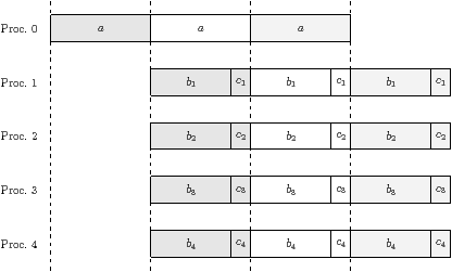
Figure 4.9 shows the worst-case example for oldest-first, from Figure 4.6(a), redrawn as a stream graph, with the kernels given labels a, b1, and so on. An execution trace is shown in Figure 4.9(b). For comparison, an optimal execution trace is shown in Figure 4.9(c). As described in Section 4.2.2, this example suffers from exhaustion: processor utilisation is poor because the oldest-first scheduler finishes the tasks from one iteration before starting the next. The next iteration starts with a single expensive kernel a, and all other processors have to wait for it to finish.
The problem is apparent in the trace—only one processor is busy just before kernel a finishes. To avoid this problem, each firing of kernel a should have started executing earlier. In contrast, every time kernel b1 finishes executing, roughly half of the processors are busy. The precise number depends on the order in which b1 through b4 and c4 finish, and on the latency in the run-time system between the time a task finishes and the thread is marked idle. Figure 4.10 is an example set of statistics after three iterations. It gives, for each kernel, the number of times that kernel has been done and the average number of threads that were busy just before it finished.
The average number of busy threads for kernel a is low, so a is probably the bottleneck. The problem can be alleviated or fixed by increasing kernel a’s priority. The following sections extend this idea into a working scheduler.
(b) Stream graph for example in Figure 4.6(a) for five processors
(b) Example execution trace for five processors (shading distinguishes iterations)
(c) Optimal execution trace for five processors (shading distinguishes iterations)
Figure 4.9: Motivation for busyness statistic
Kernel a ← b1 b2 b3 b4 c1 c2 c3 c4
Figure 4.10: Example statistics after three iterations of the program in Figure 4.9
Name Notation Initial value Description For every thread State Sj not started State: not started, busy, or idle For every kernel Adjustment ak 0 Priority adjustment for this kernel Sum busy threads tk 0 Used to calculate average busy threads Starved count sk 0 Number of times kernel was starved Non-starved count ck 0 Number of times kernel has completed without being starved
Table 4.4: Statistics for adaptive schedulers
Table 4.4 lists the small set of statistics that are maintained by the apriority and gpriority schedulers. Each worker thread starts in state not started, in which it remains, until the scheduler issues the first task to run on it. In order to avoid discriminating against kernels near the top of the stream graph during the first few iterations, processors are also considered busy if they have not executed any tasks yet. The scheduler keeps track of the number of busy threads, which is the number of threads in the not started or busy state.
Every time a task completes, the adaptive scheduler needs to update the corresponding kernel’s statistics. This must be done before any successors of the task can become ready. If the next task for the same kernel has not yet been created, the kernel is said to be starved, and the master thread could be the bottleneck. If this happens too often, there would probably be little point in increasing that kernel’s priority anyway. If the kernel is starved and there is at least one idle thread, the starved count for this kernel is increased. Otherwise, the kernel’s non-starved count is increased by one, and the sum of busy threads is increased by the current number of busy threads.
The update algorithm for apriority is called every so often to modify the priority adjustments. It happens on a worker thread at the end of complete-task. More details on the update interval are given below.
The update algorithm works as follows. First, if more than 10% of tasks were starved; that is, if ∑k sk ≥ 1/10∑k ck, the main thread is probably the bottleneck, and there is little the adaptive scheduler can do, except try to minimise overhead. In this case, the priority adjustments are left unchanged, and the interval to the next time the update algorithm is called is increased. The experiments in Section 4.4 simply use an interval of 100ms for the normal case and 500ms if more than 10% of tasks were starved. This behaviour could be made more sophisticated.
If fewer than 10% of tasks were starved, a candidate kernel is identified. The candidate has the lowest average number of busy threads. In case of ties, it is the kernel with the largest ID, which is the one nearest the bottom of the stream graph. The average number of busy threads for the candidate is compared with the average for all kernels. If it is less than 90% of the average for all kernels, then the candidate is treated as a the bottleneck kernel; otherwise, there is no clear bottleneck kernel.
The priority of the bottleneck kernel is increased by the number of kernels per iteration. In order to avoid priority inversion, if any of the candidate’s predecessors now have a lower priority than it, their priorities are increased to be the same. This procedure applies to all ancestors of the candidate. After updating any kernel adjustments, all kernels have their statistics reset: tk := 0, sk := 0, and ck := 0 for all k.
For the example in Figure 4.9, the candidate is kernel a, its average number of busy threads is 1.0, which is less than 90% of the average since the average is 3.7. Its priority adjustment is increased to eight, which correctly pipelines the program. All statistics are reset, no other priority adjustments are increased, and the program remains correctly pipelined for the rest of the execution.
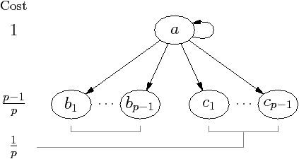
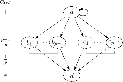
It may seem sufficient, after updating a kernel’s adjustment, to only reset the statistics for either that kernel or that kernel and its ancestors. Figure 4.11 is an counterexample to such a claim. The bottleneck is kernel a, exactly as before. After correctly increasing the priority adjustment for kernel a, kernel d will next appear to be the bottleneck. Unfortunately, updating the priority adjustment for kernel d makes all priority adjustments the same, which has the same effect as if they were all zero.
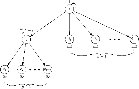
Figure 4.12 is an example that illustrates why the adaptive algorithms need to update the ancestors of the indicated kernel. Subfigure (a) is the stream graph. All kernels have multiplicity one, and cost shown outside the vertex, where p is the number of processors and є ≪ 1 is some small number much less than one. Since the only stateful kernel is the source, a, the critical path has cost 1 per iteration.
The total work per iteration is
|
so an optimal schedule on p processors requires time 1 per iteration.
Subfigure (b) is an example trace of two iterations, using the oldest-first scheduler. This requires time 2p−1/p+є/2 per iteration.
Subfigure (c) shows the busy statistics for the apriority scheduler, which is, for each kernel, the average number of busy processors just as it finishes, but before any of its predecessors wake up. The startup mechanism means that even on the first iteration, kernel a registers p busy processors. The results for b and c are clear. The value for kernel d is an average: the first kernel d that finishes sees p busy processors, the second sees p−1 busy processors, and the last sees two busy processors. The average can be found by pairing off in pairs, starting with the first and last, and each pair has average p+2/2 busy processors.
The apriority and gpriority schedulers will therefore identify kernel b as the critical path, and increase its priority. Unfortunately kernel b already always executes immediately after kernel a in the same iteration, so increasing its priority makes no difference—it is necessary also to increase the priority of kernel a.
The gpriority algorithm differs from apriority in the following ways. First, some decision has to be made about what constitutes a kernel. Second, the dependency graph between kernels is constructed at run-time, rather than being provided somehow by the compiler. Third, this kernel dependency graph may be cyclic. Fourth, there is no concept of a steady-state iteration.
A reasonable definition of a kernel is the source line of the caller of the StarSs task. For a stream program, converted using str2oss or a similar tool, this definition is consistent with apriority. When the same kernel definition is instantiated several times in a stream graph, each instantiation is treated as a different kernel. Figures 5.15 and 5.16 show the translated code for a stream program: lines 95 and 96 correspond to two different kernels with the same function definition.
To construct the kernel dependency graph, in create-task, the scheduler has to map from the task to the kernel. This can be done either by explicitly adding tags in the compiler, or hashing the address of the work function. The latter works when the work function is actually a wrapper, which is the case using the Mercurium source to source compiler for OmpSs.
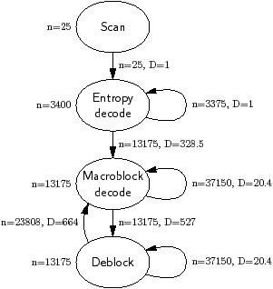
Figure 4.13 shows an example kernel dependency graph, constructed by gpriority for 25 frames of HD 1080p video through the H.264 decoder skeleton. There are four kernels, corresponding to the four stages in this H.264 decoder skeleton. This benchmark has streaming behaviour, but it is not one dimensional. Macroblock decode and Deblock iterate over a two-dimensional space.
To the left of each of kernel is shown the number of times it was called; e.g. Scan was called 25 times: once per frame. Each edge shows the number of times, n, that that dependency was seen in the PDG, and the distance, which is the average difference, D, in task number. For example, assuming that the tile width is two or more, macroblock decode usually depends on three of its neighbours: the tile to the left, with difference 1, the tile above, with difference 31, and the tile above and to the right, with difference 30.3 The average of these values is 20.7, which is close to the value that was measured. The measured distance is a little different, because some of these dependencies are missing at the image borders.
The priority of a task is equal to its kernel’s priority adjustment minus the task number, as for apriority. The priority adjustments for the kernels control the overlapping of kernels. Each kernel, however, is effectively scheduled using oldest-first, since all the tasks for the same kernel have the same adjustment. The gpriority scheduler uses the same statistics, shown in Figure 4.4, as apriority. Similarly, the bottleneck kernel is found in exactly the same manner as before.
Since there is no concept of steady-state iteration, the priority adjustment for the bottleneck kernel cannot be increased by the number of tasks per iteration. Instead, each kernel has a delta value, which is initialised to some small number. Whenever that kernel has its priority adjustment increased, it is increased by the delta, and the delta is doubled. This mechanism is rather crude, but it seems to work.
Whenever a kernel is identified as a bottleneck and its priority adjustment is increased, the adjustments of its ancestors are updated to avoid priority inversion. For example, if the adjustment of Entropy Decode is increased from zero to Δ, the adjustment of Scan would be increased from zero to Δ − 1. Unlike for apriority, this procedure takes account of the average difference in task number.
After increasing the priority adjustment for kernel k from ak to ak′ = ak + Δ, each of that kernels predecessors, p, are visited in turn. The predecessor’s priority adjustment is updated:
| ap′ = max(ap, ak + Δ − Dpk) where Dpk is the distance of the edge from p to k. |
The intuition is that priority inversion happens when a task has higher priority than a predecessor. The difference in priorities of tasks is equal to the difference in priority adjustment minus the difference in task number.
This section describes the experimental results for the schedulers described in Section 4.2.1, together with the adaptive schedulers described in Section 4.3. The implementation and results use OMP Superscalar (OmpSs), but they are not specific to it. The OmpSs compiler generates an executable that uses the Nanos++ runtime library.
The benchmarks are listed in Table 4.5. The StreamIt 2.1.1 benchmarks [GTA06] are one-dimensional stream programs written in the StreamIt language. They were converted to StarSs source code using a conversion tool, known as str2oss, described in Section 5.3.
At the time of writing, Nanos++ does not yet implement renaming, described in Section 1.4.1. If each task for a given filter were to write its output into the same temporary array, there would be output and anti-dependencies between consecutive iterations. For this reason, a command-line option was added to str2oss to expand the sizes of the temporary arrays by a given factor, n, and use the segments in round-robin order. Each unwanted dependency therefore crosses n iterations rather than one.
The experimental results include measurements of the peak memory use. This is the largest amount of memory that would be used for renaming. Since Nanos++ does not actually do renaming, the memory use was modelled by the application.
Table 4.5: Benchmarks used in the evaluation
There are four additional benchmarks written in StarSs. Check LU factorises a non-symmetrical matrix into the product of a lower-triangular and an upper-triangular matrix, without a permutation matrix: A=LU. It was taken as-is from the SMP Superscalar 2.1 distribution, including a correctness check at the end, which is the sparse matrix multiplication of L and U. Cholesky uses LAPACK and BLAS routines to perform a Cholesky decomposition: A=LLT.
The H.264 decoder skeleton has the same pattern of dependencies as an H.264 decoder using the 3D wave optimisation [MAJ+09]. The entropy decoder was unrolled by 60 macroblocks, and the macroblock decode and deblocking tasks were unrolled by four in each direction, using the standard tile shape.
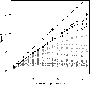
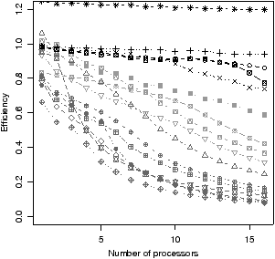
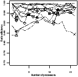
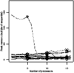
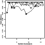
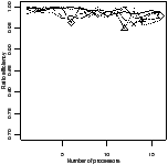
Figure 4.14 shows how well the benchmarks scale, as the number of processors varies between one and sixteen. The comparison is between the best dynamic scheduler and a serial implementation, compiled with GCC instead of the OmpSs compiler. The best scheduler is chosen independently for each data point, in order to estimate the scalability of the application itself.
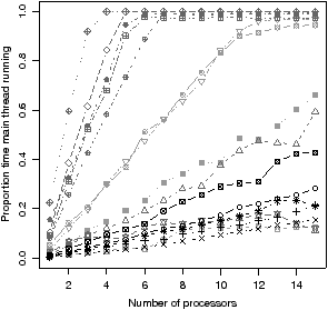
It is clear that across the benchmarks there is a wide range of scalability: filterbank scales exceptionally well. Five benchmarks have 80% or higher efficiency to sixteen cores. Other benchmarks, especially des, have poor scalability. As can be seen from Figure 4.14(c), most of the benchmarks that scale poorly have the main thread running for a large proportion of time. This shows that for these benchmarks the main thread is the bottleneck.
The reason why some benchmarks have especially poor performance is that, although the benchmarks have been optimised using kernel unrolling, they have not benefited from kernel fusion. This is because the str2oss tool described in Section 5.3 supports unrolling but not fusion. This is evidence that a partitioning algorithm like that in Section 3.2 is still beneficial, even with dynamic scheduling.
Nevertheless, the wide range of scalability means that the results of this section are applicable both to benchmarks that scale well and benchmarks that scale poorly.
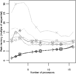
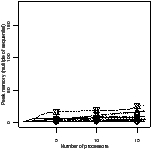
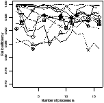
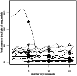
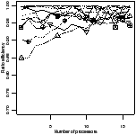
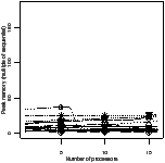
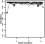
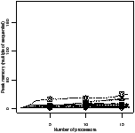
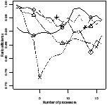
Figure 4.15(a) and (b) show, for each scheduler, the average utilisation and average peak memory use, where the average is taken across all streaming benchmarks. The non-streaming benchmarks were excluded, since they are not supported by wave and apriority. The memory use is the multiple of that required by the sequential version of the benchmark. It includes all data regions used by the benchmark and renamed by the run-time, but it excludes data structures used by the run-time itself; for example to store the PDG.
Three heuristics have consistently poor average performance, between 7% and 10% worse than oldest and the two adaptive policies. These are botlev, crit, and mdesc; all of which suffer due to the overhead of recalculating the bottom level or the number of descendants as the PDG is built.
The averaged peak memory footprint shows a wide range: toplev is particularly prone to poor back pressure, causing excessive average memory use. The oldest, apriority and gpriority schedulers have considerably lower memory use than the others, since these schedulers tend to overlap few stream program iterations.
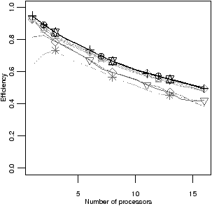
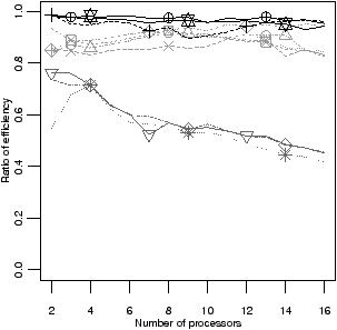
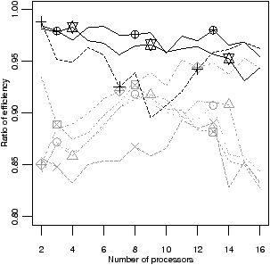
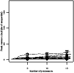
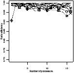
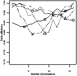
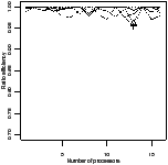
Figure 4.15(c) and (d) compares the robustness of the schedulers. In Figure 4.15(c), each data point is the worst case ratio of efficiency, which is the efficiency of the scheduler, divided by the efficiency of the best scheduler, for that benchmark and number of processors. The worst case is found across the streaming benchmarks. A value of 1.0 on the y-axis therefore indicates that, for all benchmarks, the scheduler achieves the best performance seen. Figure 4.16 shows the same results, but magnified to show only the efficiency of the more robust schedulers.
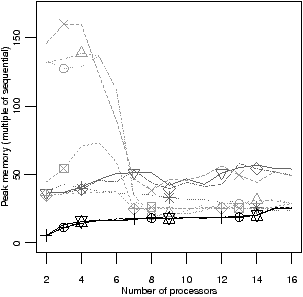
Figure 4.15(d) is the worst case memory use, as a multiple of the sequential version. As before, the worst case is found across all streaming benchmarks.
As before, botlev, crit and mdesc are clearly the worst-performing schedulers, again due to the overhead of calculating the bottom level or number of descendants.
The only robust schedulers are the adaptive schedulers, apriority and gpriority. Of the non-adaptive schedulers, oldest is best performing overall, but its worst efficiency is up to 8% lower.
The worst case peak memory footprint shows a wider range: toplev, fifo, and lifo have excessive memory use for certain benchmarks. The remaining heuristics have intermediate memory use, which is considerably higher than that of oldest, apriority, and gpriority. Compared with oldest, the two adaptive schedulers use a negligible amount of additional memory.
This section compares the efficiency and memory use of the six best schedulers. These are fifo, oldest, toplev, wave, and the two adaptive schedulers: apriority and gpriority. The other schedulers were seen to have poor robustness and average performance.
Figure 4.17 shows the experimental results for the StreamIt benchmarks. There are two plots for each scheduler. The first is the ratio of efficiency: the efficiency of that scheduler divided by the efficiency of the best scheduler for the same benchmark and number of processors. The y axis has been expanded to show greater detail—no points were lost in doing so. The second plot is the peak memory use, as a multiple of the sequential version.
The apriority scheduler has the highest efficiency and lowest memory use. The gpriority scheduler has slightly lower efficiency due to the greater overhead, and the same low memory use.
Figure 4.18 shows the experimental results for the non-StreamIt benchmarks. The wave and apriority schedulers were excluded, since they both require regular stream programs, so do not support these benchmarks. It was not possible to determine the memory footprint, because Nanos++ does not currently implement renaming. As described in Section 4.4, the renaming memory footprint was modelled by the application, and this was only implemented for the StreamIt benchmarks.
The gpriority scheduler has the best efficiency and memory use overall.
This chapter introduced two new low-complexity adaptive dynamic scheduling algorithms for stream-like programs. Many existing scheduling algorithms, listed in Table 4.1, either schedule the whole program in advance, or they need to know the execution time of every task in advance, or they are too slow.
The scheduling algorithms in this chapter have better average and worst-case performance than all the scheduling algorithms in Table 4.2. The scheduling overhead at run-time is similar to that of oldest-first. They take advantage of the stream graph representation, by giving each kernel in the stream graph its own priority adjustment.